parid
parid.Rmd
library(parid)
#> Loading required package: ggplot2
#> parid, version 1.0, (C) 2023 LAP&P Consultants BV. See COPYING for license info
Introduction
This is an example showing how to use the parid package. The example defines a nonlinear mixed effects model, and analyzes its parameter identifiability using three methods:
- the Sensitivity Matrix Method (SMM)
- the Fisher Information Matrix Method (FIMM)
- the Aliasing Method
This example assumes familiarity with mixed effects modeling. More details on the methods and on parameter identifiability in general can be found here. R code running this same example can be found in the package, at tests/example.R.
Model definition
The model is a one-compartmental linear PK model with absorption and a single oral dose. The model parameters are clearance (CL), volume (V), the absorption rate constant (Ka) and optionally the bio-availability (F); they are defined in terms of underlying structural and inter-individual parameters. In this example, inter-individual variability is included on clearance. The output is the concentration, which is modeled with an additive error.
The expected outcome is that this model will not be identifiable because the bio-availability cannot be determined independently from the clearance and volume. If the bio-availability is fixed, then the model should be identifiable.
The next lines of code create four functions defining this model:
-
model: returns the differential equations describing the time evolution of the model. The input arguments are the timet, the current statey(i.e., the amounts in the depot and central compartments), and the model parametersp. -
p: returns the model parameters as function of the structural parametersthetaand inter-individual parameterseta. The dose is also included here. In general, any covariates could be included. For all parameters except CL, the value is simply the value of the corresponding structural parameter. -
init: returns the initial values of the state variables, as function of the model parametersp. In this example, the depot is initialized to the bio-available fraction of the dose, and the central compartment to zero. -
output: returns the model output, that is the concentration (with residual error), as function of the statey, the model parameterspand the residual erroreps.
model      <- function(t, y, p) { c(-p[["Ka"]]*y[["x1"]], p[["Ka"]]*y[["x1"]] - p[["CL"]]/p[["V"]] * y[["x2"]]) }
p          <- function(theta, eta) { c(Ka = theta[["TVKa"]], CL = theta[["TVCL"]] * exp(eta[["iCL"]]),
                                       V = theta[["TVV"]], F = theta[["TVF"]], Dose = theta[["TVDose"]])  }
init       <- function(p) { c("x1" = p[["F"]] * p[["Dose"]], "x2" = 0) }
output     <- function(y, p, eps) { y[["x2"]] / p[["V"]] + eps[["addErr"]] }
Parameter definition
The next piece of code sets the values for the structural parameters
(theta). Some parameters can be considered as fixed. This
is typically done for covariates (in this example the dose). The vectors
vartheta1 and vartheta2 define two variants;
the first one also sets the bio-availability F as fixed, the second one
keeps it variable.
Variance matrices omega and sigma are
defined for the random variables eta and eps,
respectively. Their row and column names should be the same as the ones
used in the model definition. These matrices are the random-effects
parameters.
theta      <- c("TVKa" = 1, "TVCL" = 0.2, "TVV" = 2, "TVF" = 0.7, "TVDose" = 10)
vartheta1  <- setdiff(names(theta), c("TVDose", "TVF"))     # Bioavailability F is fixed
vartheta2  <- setdiff(names(theta), "TVDose")               # Bioavailability F is variable
omega      <- diag(0.3, nrow = 1)
colnames(omega) <- row.names(omega) <- c("iCL")
sigma      <- diag(0.1, nrow = 1)
colnames(sigma) <- row.names(sigma) <- c("addErr")
Sampling times
The vector times contains the sampling times. The
initialization (in this example, the time of dosing) is always set to
zero.
times <- seq(0, 10, 1)Variational equations
As a first step in the calculation, the variational equations are
solved. This is done two times, once for every setting of fixed
parameters as defined above, and will create data frames
vareq1 and vareq2 containing the derivatives
of the model output (the concentration) with respect to the structural
and random-effects parameters, evaluated at the sample times. The
derivatives are plotted over time. The plot functions have options
controlling which derivatives are plotted. See their documentation for
details.
vareq1 <- calcVariationsFim(model = model, p = p, init = init, output = output, times = times, symbolic = TRUE,
                           theta = theta, nmeta = colnames(omega), nmeps = colnames(sigma), vartheta = vartheta1)
plotVariations(vareq1)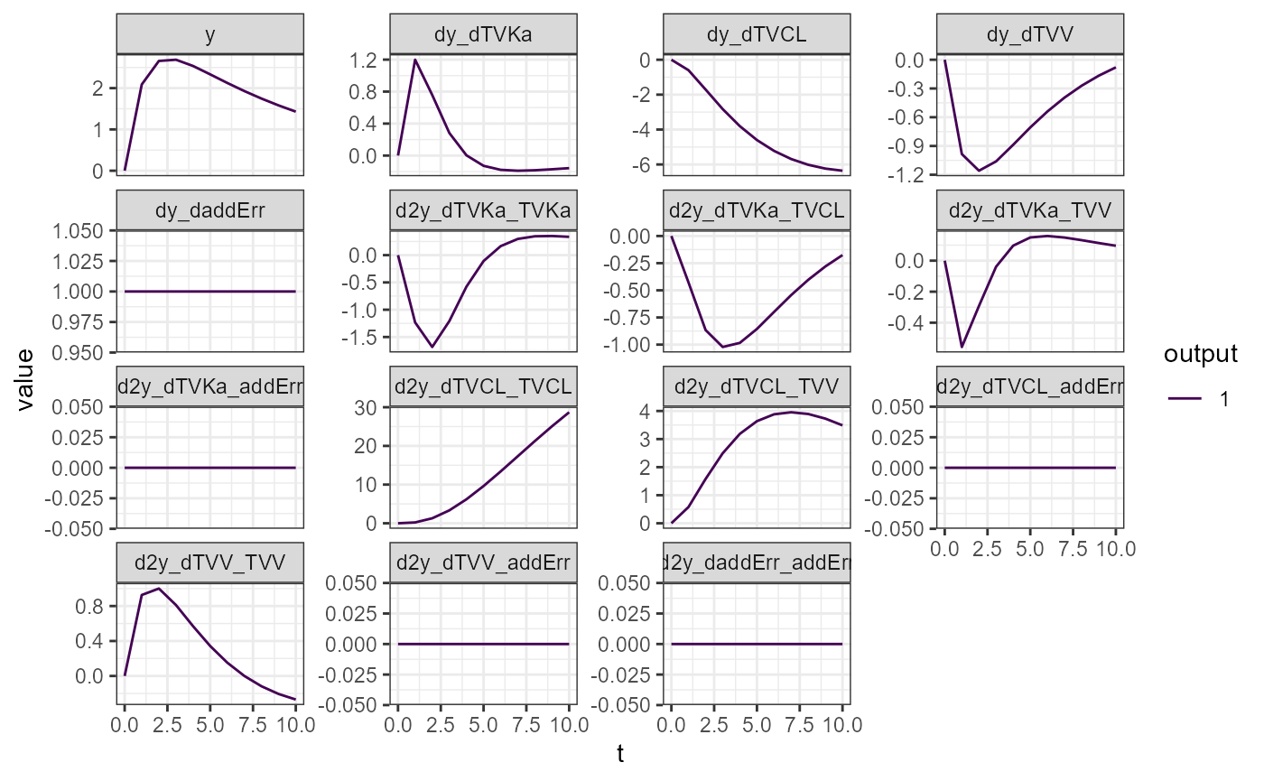
vareq2 <- calcVariationsFim(model = model, p = p, init = init, output = output, times = times, symbolic = TRUE,
                            theta = theta, nmeta = colnames(omega), nmeps = colnames(sigma), vartheta = vartheta2)
plotVariations(vareq2)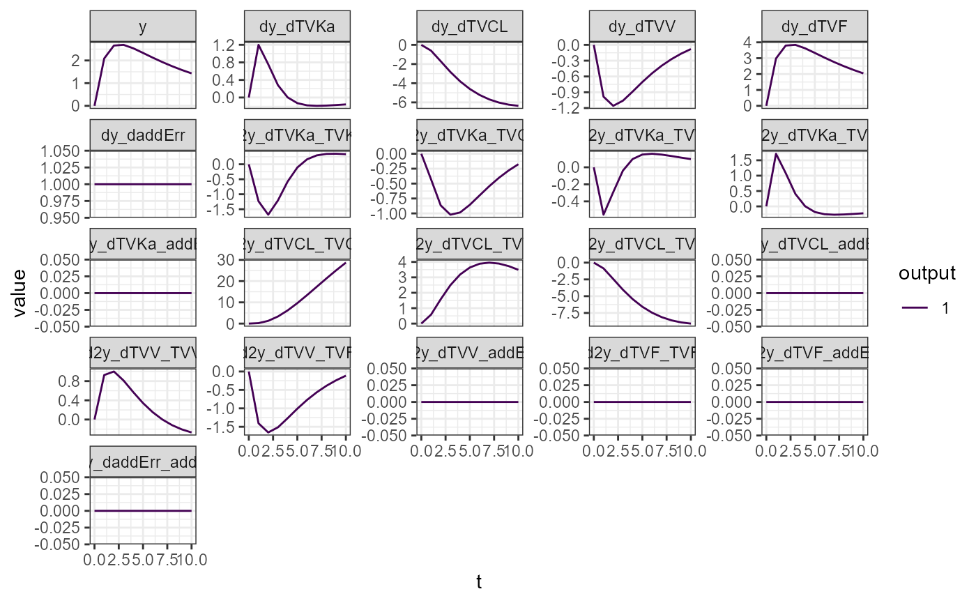
Compute and plot Sensitivity Matrix Method (SMM) results
SMM results are generated from the variational matrices
vareq1 and vareq2 using the function
calcSensitivityFromMatrix. The outputs
argument controls which SMM indicators are computed. They are (more details):
- The null space dimension
N. This is a categorical indicator, equal to the number of unidentifiable directions. So 0 means identifiable, and larger than 0 means unidentifiable. - The skewing angle
A. This is a continuous indicator, taking values between 0 and 1, where 0 means unidentifiable, 1 means identifiable. IfAis close to 0 then the model is close to unidentifiable. - The unidentifiable directions
R. This lists the parameter directions in which the model is unidentifiable. The number of directions equalsN. - The minimal parameter relations
Mand the M-norm given by itsnormattribute. The M-norm is a continuous indicator, taking values between 0 and 1, where 0 means unidentifiable, 1 means identifiable. If the M-norm is close to 0 then the model is close to unidentifiable. For small M-norms, the vectorMcontains the parameter direction in which the model is unidentifiable. - The least identifiable parameter norms (L-norms)
L. This is a vector of continuous indicators, one for each parameter, taking values between 0 and 1, where 0 means unidentifiable, 1 means identifiable. If a component ofLis close to 0 then that parameter is close to unidentifiable.
The results are displayed and graphed. The first variant, where the
bio-availability F was fixed, is identifiable, as can be seen from the
output of simplifySensitivities(sens1): the null space
dimension N is 0, and the skewing angle, M-norm and L-norms
are all large.
sens1 <- calcSensitivityFromMatrix(outputs = list("N", "A", "R", "M", "L"), df = vareq1, vars = vartheta1)
simplifySensitivities(sens1)
#> $N
#> [1] 0
#>
#> $A
#> [1] 0.6668127
#>
#> $R
#>
#> TVKa
#> TVCL
#> TVV
#>
#> $M
#>             [,1]
#> TVKa  0.75420019
#> TVCL -0.07767148
#> TVV   0.65203467
#> attr(,"norm")
#> [1] 0.1814101
#>
#> $L
#>       TVV      TVCL      TVKa
#> 0.4485372 0.5462389 0.5542248
plsens1 <- plotSensitivities(sens1)
plsens1 <- lapply(plsens1[lengths(plsens1) > 0], function(pl) pl + theme_bw(base_size = 8))
cowplot::plot_grid(plotlist = plsens1, nrow = 1)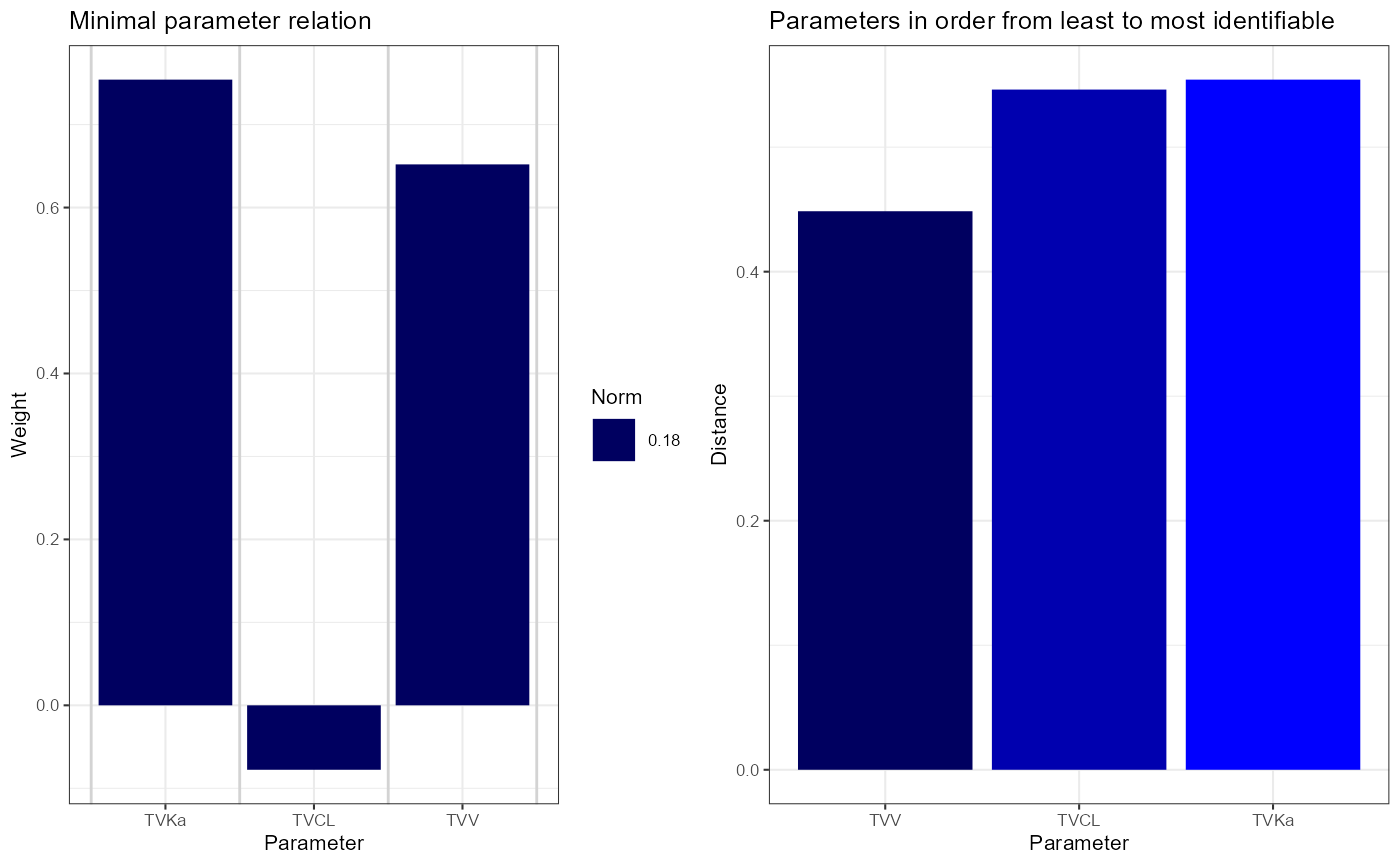
The second variant, where F was variable, is not identifiable, see
the output of simplifySensitivities(sens2): the null space
dimension is 1, and the skewing angle, M-norm and L-norms are all small
or even zero. The indicators R and M find a
relation involving F, CL and V, as expected.
sens2 <- calcSensitivityFromMatrix(outputs = list("N", "A", "R", "M", "L"), df = vareq2, vars = vartheta2)
simplifySensitivities(sens2)
#> $N
#> [1] 1
#>
#> $A
#> [1] 0.002006091
#>
#> $R
#>           [,1]
#> TVKa 0.0000000
#> TVCL 0.0939682
#> TVV  0.9396820
#> TVF  0.3288887
#>
#> $M
#>           [,1]
#> TVKa 0.0000000
#> TVCL 0.0939682
#> TVV  0.9396820
#> TVF  0.3288887
#> attr(,"norm")
#> [1] 0
#>
#> $L
#>       TVF       TVV      TVCL      TVKa
#> 0.0000000 0.0000000 0.0000000 0.5542248
plsens2 <- plotSensitivities(sens2)
plsens2 <- lapply(plsens2[lengths(plsens2) > 0], function(pl) pl + theme_bw(base_size = 8))
cowplot::plot_grid(plotlist = plsens2, nrow = 1)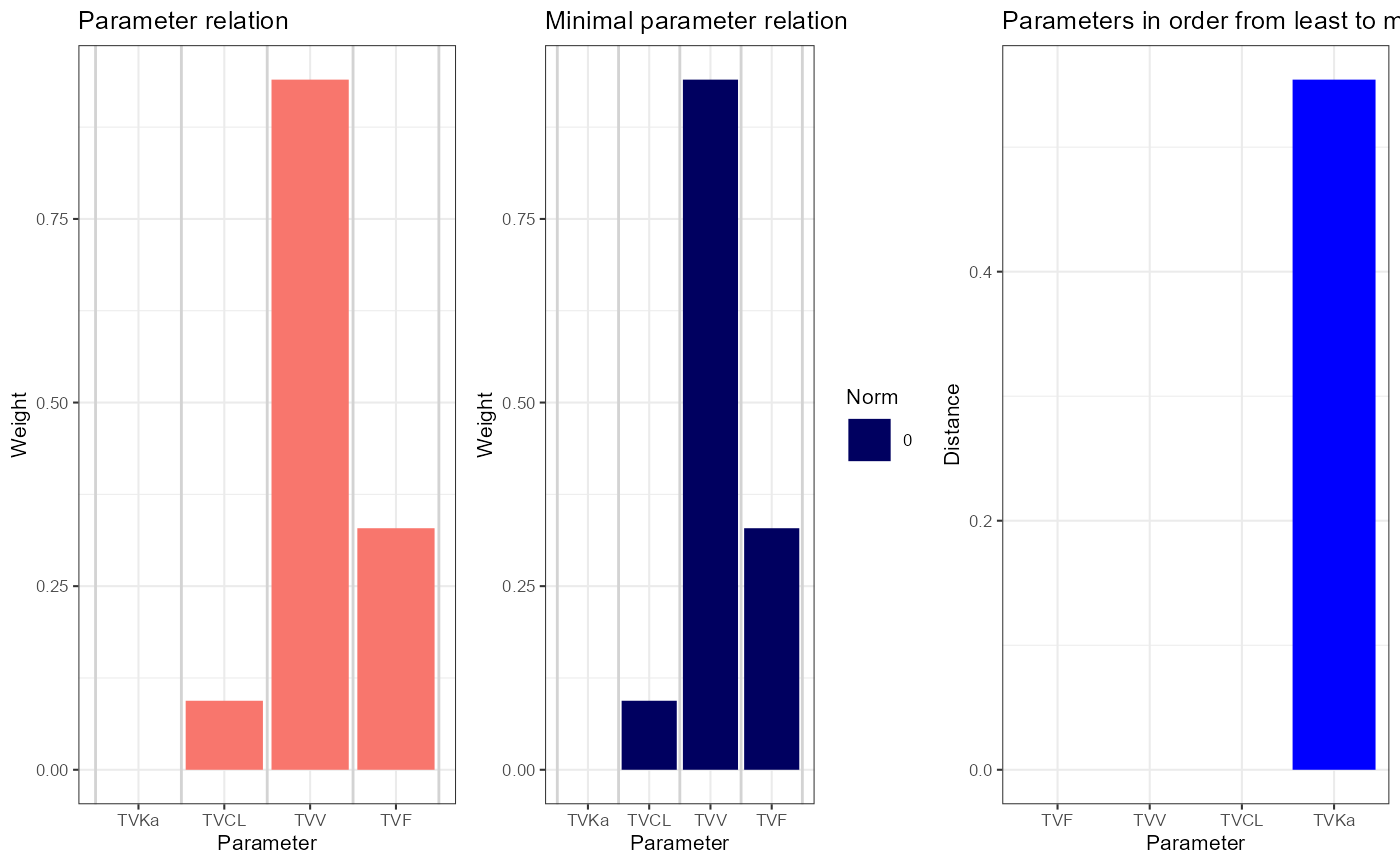
Compute and plot Aliasing Method results
The results are generated from the variational matrices
vareq1 and vareq2 using the function
calcAliasingFromMatrix. The results are displayed and
graphed. Both variants are identifiable, as aliasing scores are quite
low. This is because the aliasing method can only find identifiability
problems involving two parameters, and not three.
alia1 <- calcAliasingScoresFromMatrix(df = vareq1, vars = vartheta1)
plalia1 <- plotAliasing(alia1, elt = c("S", "T"))
cowplot::plot_grid(plotlist = plalia1, nrow = 1)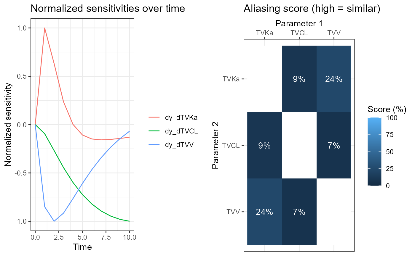
alia2 <- calcAliasingScoresFromMatrix(df = vareq2, vars = vartheta2)
plalia2 <- plotAliasing(alia2, elt = c("S", "T"))
cowplot::plot_grid(plotlist = plalia2, nrow = 1)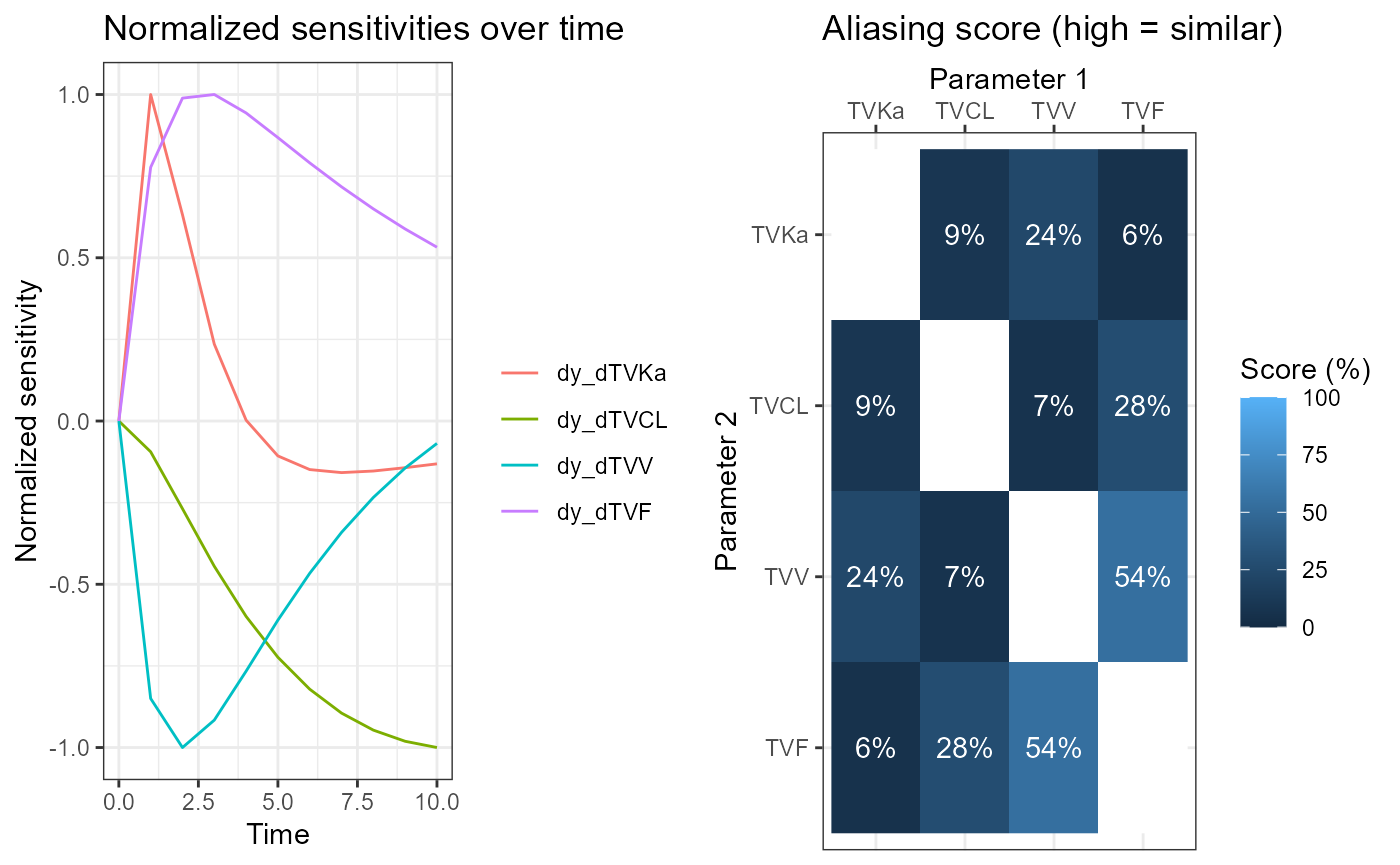
Compute and plot Fisher Information Matrix Method (FIMM) results
FIMM results are generated from the variational matrices
vareq1 and vareq2 using the functions
calcFimFromMatrix and fimIdent, that compute
the Fisher Information Matrix (FIM) and the parameter identifiability
indicators, respectively. The indicators are (more details):
- Categorical identifiability
identifiable. This isTRUEif all curvatures are 0 and the model is identifiable, andFALSEif there are positive curvatures and the model is unidentifiable. The curvatures describe the objective function value (OFV) surface as function of the parameters. - The number of 0 curvatures
nDirections. This is a categorical indicator counting the number of 0 curvatures. - The parameter vectors
directionscorresponding to the curvatures, in order of increasing curvature. For zero (or small) curvatures, they indicate the directions in parameter space of (near) unidentifiability. - The curvature values
curvaturesof the OFV surface. Zero values correspond to unidentifiability, small values indicate near unidentifiability. - The index
jumpof the highest change in curvature value. - The estimated standard error
se, calculated from the FIM. - The estimated relative standard error
rse, calculated from the FIM.
The results are displayed. The first variant, where the
bio-availability F was fixed, is identifiable: all curvatures are high.
The options relChanges = TRUE and ci = 0.95
imply that the directions show the relative percentage
changes corresponding to an insignificant increase (at 95%) in objective
function of at most 3.84, for the given number of subjects. They are all
below 50%.
fim1 <- calcFimFromMatrix(df = vareq1, omega = omega, sigma = sigma, vartheta = vartheta1)
fimres1 <- fimIdent(fim = fim1, curvature = 1e-10, relChanges = TRUE, ci = 0.95, nsubj = 30)
simplifyFimIdent(fimres1)
#> $identifiable
#> [1] TRUE
#>
#> $nDirections
#> [1] 0
#>
#> $directions
#>              [,1]       [,2]       [,3]         [,4]     [,5]
#> TVKa    9.9061084 -8.6678631 -2.9435682  -0.12214659  0.00000
#> TVCL   -6.0881243 -0.3264183  0.1793294 -16.80599830  0.00000
#> TVV     4.0494263 -3.0153337  1.9606156  -0.03457756  0.00000
#> iCL    45.2711270 33.0420632 -0.6269551  -0.57003282  0.00000
#> addErr -0.1127873 -0.1378980  0.0251975   0.05610669 16.00194
#>
#> $curvatures
#> [1]   109.8634   183.1313  1595.4680  3385.5471 15002.0161
#>
#> $jump
#> [1] 2
#>
#> $se
#>       TVKa       TVCL        TVV        iCL     addErr
#> 0.37694626 0.09992565 0.30271768 0.46993184 0.04472136
#>
#> $rse
#>      TVKa      TVCL       TVV       iCL    addErr
#>  37.69463  49.96282  15.13588 156.64395  44.72136
The second variant, where F was variable, is not identifiable, as the
first curvature is close to zero. It finds a relation involving F, CL
and V in directions, as expected. The relative changes are
very large, indicating that the parameters can change by a large factor
without significantly changing the OFV.
fim2 <- calcFimFromMatrix(df = vareq2, omega = omega, sigma = sigma, vartheta = vartheta2)
fimres2 <- fimIdent(fim = fim2, curvature = 1e-10, relChanges = TRUE, ci = 0.95, nsubj = 30)
#> Warning in FisherInfo::fimIdent: SE's and RSE's cannot be calculated because FIM cannot be inverted. I will set them to NA, and continue without them.
simplifyFimIdent(fimres2)
#> $identifiable
#> [1] FALSE
#>
#> $nDirections
#> [1] 1
#>
#> $directions
#>             [,1]       [,2]         [,3]         [,4]        [,5]      [,6]
#> TVKa           0  7.0481967  11.48509526  -0.47008081 -0.36997026   0.00000
#> TVCL   -70517721 -8.4600755  -4.92646955 -16.70180859  1.37943161   0.00000
#> TVV    -70517721  0.3837179   0.44188540   0.21666273  0.28984508   0.00000
#> TVF    -70517721 -2.4417729  -3.20506697  -0.40526242 -2.47868897   0.00000
#> iCL            0 52.9879893 -18.27022014  -0.66179776 -0.07046264   0.00000
#> addErr         0 -0.1496521   0.09507588   0.06271155  0.06099013 -16.00182
#>
#> $curvatures
#> [1] 1.705303e-12 1.244213e+02 2.276623e+02 3.287036e+03 1.079053e+04
#> [6] 1.500206e+04
#>
#> $jump
#> [1] 1
#>
#> $se
#>   TVKa   TVCL    TVV    TVF    iCL addErr
#>     NA     NA     NA     NA     NA     NA
#>
#> $rse
#>   TVKa   TVCL    TVV    TVF    iCL addErr
#>     NA     NA     NA     NA     NA     NA